Overview
Traditional mobile robot navigation systems, such as SLAM-based architectures, rely on building dense obstacle maps from expensive high-resolution sensors . These methods are computationally intensive and slow to update dynamically .
This project implements an end-to-end mapless motion planner for differential-drive mobile robots using continuous Deep Reinforcement Learning . Based on Asynchronous Deterministic Policy Gradient (ADDPG), the model takes a highly compressed 14-dimensional state representation—comprising 10 sparse laser range samples, 2D relative target positions in polar coordinates, and previous velocity commands—and outputs smooth continuous linear and angular velocity commands . Trained entirely within a simulated environment ( Pybullet), the learned policy directly transfers to physical robotic hardware (Kobuki-based TurtleBot) without any real-world fine-tuning . This is taken from the paper Virtual-to-Real Deep Reinforcement Learning: Continuous Control of Mobile Robots for Mapless Navigation by Tai et al.
State & Action Space Formulation
The mapless navigation task is modeled as a continuous Markov Decision Process (MDP) . The input state vector $s_t \in \mathbb{R}^{14}$ is constructed at each control step by concatenating three distinct observations :
\[s_t = \begin{bmatrix} x_t & v_{t-1} & p_t \end{bmatrix}\]- Sparse Laser Readings ($x_t \in \mathbb{R}^{10}$): 10-dimensional sparse laser range findings sampled at fixed angles between $-90^\circ$ and $+90^\circ$, normalized to $[0, 1]$ .
- Previous Control Inputs ($v_{t-1} \in \mathbb{R}^2$): Continuous linear and angular velocities from the preceding step $(v_{t-1}, \omega_{t-1})$ .
- Relative Target Position ($p_t \in \mathbb{R}^2$): Target destination represented in 2D polar coordinates (distance $r_t$ and relative heading angle $\phi_t$) with respect to the robot’s local frame .
The action vector $a_t = [v_t, \omega_t]^T \in \mathbb{R}^2$ commands continuous velocities bounded by physical vehicle constraints :
- Linear Velocity: $v_t \in [0, 0.5]\text{ m/s}$
- Angular Velocity: $\omega_t \in [-1.0, 1.0]\text{ rad/s}$
Continuous Control via Asynchronous DDPG (ADDPG)
To accelerate sample generation without requiring multiple parallel simulation environments, sample collection is decoupled into dedicated asynchronous background threads while maintaining a centralized off-policy replay buffer $\mathcal{D}$ .
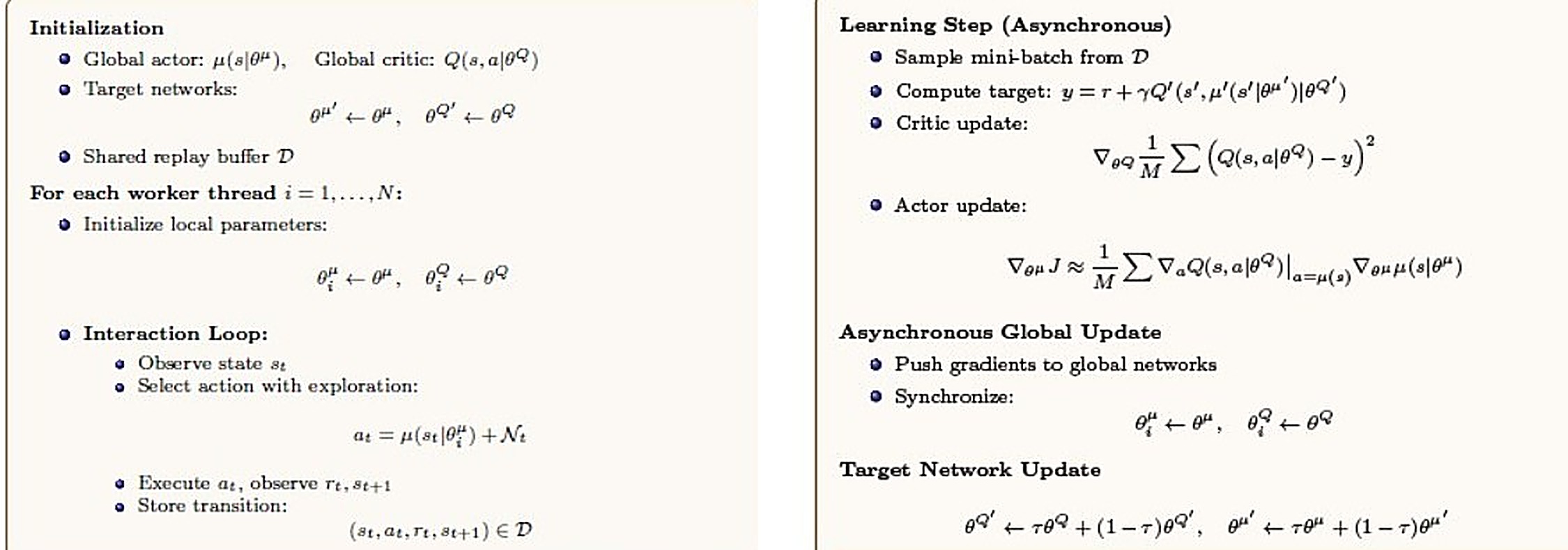
Figure 1: Asynchronous DDPG (ADDPG) training algorithm pseudocode.
Loss Formulations
The Critic Network $Q(s, a \mid \theta^Q)$ is trained as a regression problem: it minimizes the Mean Squared Bellman Error (MSBE) between its own prediction and a bootstrapped TD target $y_i$, built from each sampled transition’s reward plus the discounted value that the target networks assign to the next state and the next action the target actor would take there. Using separate, slowly-tracking target networks ($\theta^{\mu’}$, $\theta^{Q’}$) to compute $y_i$ — instead of the online networks currently being updated — decouples the regression target from the parameters chasing it, which is what keeps this bootstrapped update stable rather than diverging:
\[L(\theta^Q) = \frac{1}{M} \sum_{i=1}^{M} \left( Q(s_i, a_i | \theta^Q) - y_i \right)^2\] \[y_i = r_i + \gamma Q'\left(s'_{i}, \mu'(s'_{i} | \theta^{\mu'}) \middle| \theta^{Q'}\right)\]The Actor Network $\mu(s \mid \theta^\mu)$ has no target label of its own — instead it is nudged in whatever direction makes the critic’s output larger. Concretely, the critic’s gradient with respect to the action, $\nabla_a Q(s,a \mid \theta^Q)$, is evaluated at the action the actor would currently take, then backpropagated through the actor’s own parameters via the chain rule. This is the Deterministic Policy Gradient — a policy update that borrows the critic as a differentiable proxy for “how good was that action”:
\[\nabla_{\theta^\mu} J \approx \frac{1}{M} \sum_{i=1}^{M} \left. \nabla_a Q(s, a | \theta^Q) \right|_{a=\mu(s_i)} \nabla_{\theta^\mu} \mu(s_i | \theta^\mu)\]Both updates are computed off-policy from mini-batches drawn out of the shared replay buffer $\mathcal{D}$, which the $N$ asynchronous worker threads in Figure 1 keep filling concurrently. Rather than being copied outright, the target networks $\theta^{\mu’}, \theta^{Q’}$ are then nudged toward the online networks with a small soft-update rate $\tau$, so the bootstrapped targets drift slowly instead of jumping step to step.
Reward Function Design
The step reward function $r(s_t, a_t)$ guides target-reaching behavior while penalizing obstacle proximity :
\[r(s_t, a_t) = \begin{cases} r_{\text{arrive}} & \text{if } d_t < c_d \text{ (Target Reached)} \\ r_{\text{collision}} & \text{if } \min(x_t) < c_o \text{ (Collision Hazard)} \\ c_r (d_{t-1} - d_t) & \text{otherwise (Progress Reward)} \end{cases}\]| Hyperparameter | Description | Value |
|---|---|---|
| $r_{\text{arrive}}$ | Terminal success reward | $+15.0$ |
| $r_{\text{collision}}$ | Terminal failure penalty | $-15.0$ |
| $c_r$ | Distance reduction scaling multiplier | $2.5$ |
| $c_d$ | Terminal arrival tolerance radius | $0.25\text{ m}$ |
| $c_o$ | Minimum clearance distance threshold | $0.15\text{ m}$ |
Network Architecture & Pseudocode
The policy network processes the 14-dimensional state vector through parallel dense layers before generating bounded velocity signals .
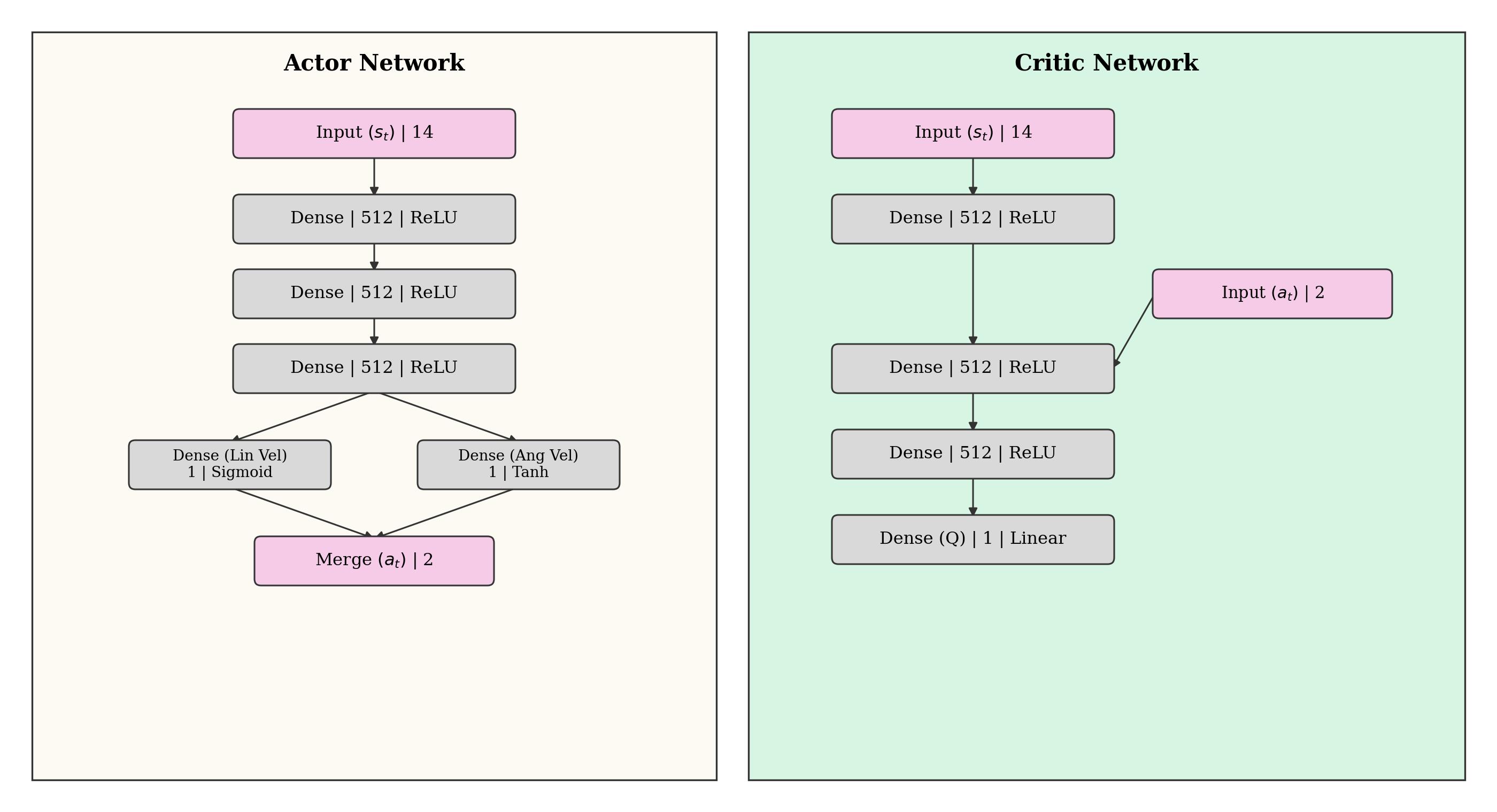
Figure 2: Network structure and layer configuration breakdown.
Visualizations & Demonstration Video
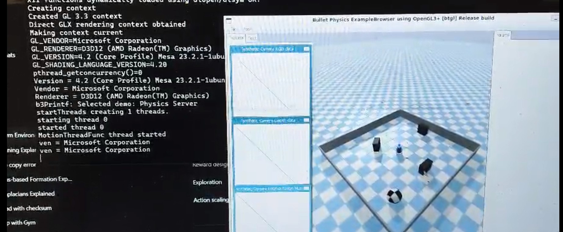
The trained ADDPG policy was evaluated across complex simulated arenas in Pybullet .
Simulation Demonstration: Continuous control mapless navigation in Pybullet indoor environments.
Experimental & Benchmark Results
The performance of the continuous Deep-RL agent was benchmarked against traditional map-based navigation stack components (Move Base) in simulated test layouts and real-world deployment evaluation :
| Planner Model | Map Required | Max Control Frequency | Execution Stability | Sim-to-Real Transfer |
|---|---|---|---|---|
| Move Base (Full Laser) | Yes | $\approx 14\text{ Hz}$ | Optimal Path | N/A (Requires Full Map) |
| Move Base (10-D Sparse) | Yes | $\approx 14\text{ Hz}$ | Failed at narrow corridors | Failed (Cost-map errors) |
| Deep-RL (Env-1 Policy) | No | $\approx 100\text{ Hz}$ | Collision-Free | Poor Generalization |
| Deep-RL (Env-2 Policy) | No | $\mathbf{\approx 100\text{ Hz}}$ | Smooth & Highly Robust | 100% Zero-Shot Success |
Critical Performance Metrics
- Control Latency: Inference time per action query is $\approx 1\text{ ms}$, achieving a $7\times$ speedup over traditional local trajectory planners ($\approx 14\text{ Hz}$) .
- Sensor Reduction: Functionally replaces dense 2D LiDAR scans with 10 discrete angular distance beams without sacrificing obstacle avoidance capabilities .
- Emergent Behaviors: Autonomous rotational recovery maneuvers naturally emerged from the trained policy when navigating tightly constrained passages .
Key Takeaways
- Successfully developed an end-to-end mapless navigation pipeline leveraging continuous Deep-RL via Asynchronous DDPG (ADDPG) .
- Proved that an abstracted 14-dimensional state representation effectively bridges the simulation-to-reality gap without fine-tuning on real hardware .
- High inference rates ($\approx 100\text{ Hz}$) enable reactive collision avoidance under real-time execution constraints .
- Future work involves integrating Recurrent Neural Network layers (LSTM/GRU) to mitigate trajectory tortuosity caused by partial observability .