Overview
In mobile robotics, motion planning is formulated in configuration space (C-space) rather than directly in the physical workspace. The configuration space represents every possible pose of a robot as a point in a higher-dimensional space . For the differential-drive TurtleBot, C-space modeling provides a rigorous mathematical framework for navigation, planning, and control.
This project implements and evaluates nonholonomic trajectory planning strategies for a differential-drive TurtleBot operating in obstacle-laden environments. We contrast deterministic grid-based planning (A*) against probabilistic sampling-based planning (RRT), dynamic obstacle inflation via Minkowski sums, and robust trajectory execution using ROS-integrated localization and trajectory tracking controllers.
Configuration Space & Kinematic Modeling
Configuration Space of TurtleBot
The TurtleBot operates on a planar surface and can both translate and rotate. Its configuration is defined by three variables:
\[q = (x, y, \theta)\]where $x$ and $y$ represent the robot’s position in the plane, and $\theta$ represents the robot’s orientation (heading angle). Thus, the configuration space is $\mathcal{C} = \mathbb{R}^2 \times S^1$. The position lies in two-dimensional Euclidean space ($\mathbb{R}^2$), while orientation lies on a circle ($S^1$), making the configuration manifold mathematically equivalent to the Lie group $SE(2)$.
Kinematic Model & Constraints
The TurtleBot is a differential-drive robot subject to nonholonomic constraints :
\[\dot{x} = v \cos(\theta)\] \[\dot{y} = v \sin(\theta)\] \[\dot{\theta} = \omega\]The system is subject to the continuous zero-lateral-velocity constraint:
\[\dot{y}\cos(\theta) - \dot{x}\sin(\theta) = 0\]This constraint prevents instantaneous sideways motion; the robot must reorient itself before changing direction . Furthermore, because $\mathcal{C} = \mathbb{R}^2 \times S^1$ is a smooth three-dimensional manifold with angular periodicity, special consideration is required during state sampling and interpolation . Despite these nonholonomic constraints, the system is small-time locally controllable, allowing arbitrary poses in free space to be reached via sequences of forward motions and rotations .
Configuration Space Obstacles & Free Space Construction
Let $\mathcal{O}$ represent obstacle regions in the physical workspace . The corresponding C-space obstacle region $\mathcal{C}_{\text{obs}}$ is defined as :
\[\mathcal{C}_{\text{obs}} = \{q \in \mathcal{C} \mid \text{the robot at configuration } q \text{ intersects } \mathcal{O}\}\]Assuming a circular disk approximation for the TurtleBot:
- Workspace obstacles are inflated by the robot’s radius using Minkowski sum operations .
- $\mathcal{C}_{\text{obs}} = (\text{inflated workspace obstacles}) \times S^1$ .
- Free configuration space is defined as $\mathcal{C}_{\text{free}} = \mathcal{C} \setminus \mathcal{C}_{\text{obs}}$ .
The trajectory generation goal is to establish a continuous trajectory $\gamma(t) \in \mathcal{C}_{\text{free}}$ for $0 \le t \le 1$ such that $\gamma(0) = q_{\text{start}}$ and $\gamma(1) = q_{\text{goal}}$, while respecting differential kinodynamic limits .
Decision-Making & Path Planning Algorithms
Two core spatial path-planning strategies were implemented and benchmarked :
1. A* Planner (Grid-Based Search)
A deterministic graph-search planner using cost function evaluation $f(n) = g(n) + h(n)$, where $g(n)$ is the exact path cost from start to node $n$, and $h(n)$ is an admissible heuristic . Implemented in astar_planner.py, it guarantees resolution optimality, generating shortest-path grid trajectories .
2. Rapidly-Exploring Random Tree (RRT Planner)
A probabilistic, sampling-based planner implemented in RRT_Planner.py . RRT rapidly explores high-dimensional C-spaces by incrementally growing a search tree toward randomly sampled states $q_{\text{rand}} \in \mathcal{C}_{\text{free}}$ . It is probabilistically complete and explores open spaces quickly, though raw paths tend to be non-optimal and jagged .
Visualizations & Experimental Demos
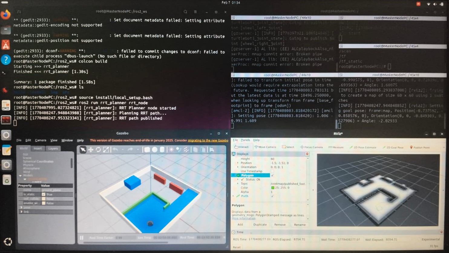
The generated global paths were executed on the TurtleBot platform via ROS integration .
Live Demonstration: A* Path Planner running on TurtleBot .
Simulation Demonstration: Full C-Space Navigation Trajectory in Gazebo/Webots Environment.
Simulation & Benchmark Results
Performance metrics were collected across 5 test runs per planner in the target environment :
| Metric | A* Planner (Average) | RRT Planner (Average) |
|---|---|---|
| Time to Goal | 42.5 seconds | 48.2 seconds |
| Path Length | 8.42 meters | 10.15 meters |
| Min. Distance to Obstacle | 0.12 meters | 0.25 meters |
| Success Rate | 100% | 80% (Occasional failures) |
Sim-to-Real Gap Analysis & Hardware Integration
Deploying planned paths to physical hardware introduced discrepancies between simulation assumptions and real-world execution :
- Wheel Slip & Kinematic Drift: Real motor wheel slip degraded dead-reckoning accuracy . This was corrected by integrating Adaptive Monte Carlo Localization (AMCL) over laser scan data .
- Obstacle Safety Margins: Imperfection in real-world wall alignment required dynamic tuning of the
inflation_radiuswithin the costmap generation node . - Processing Latency: Processing overhead on the Raspberry Pi onboard unit created execution lag . This was compensated by dynamically adjusting the lookahead distance within the Pure Pursuit path-tracking controller .
Key Takeaways
- Developed analytical C-space models incorporating nonholonomic $SE(2)$ differential constraints for TurtleBot navigation .
- Implemented and benchmarked grid-search (A*) vs. sampling-based (RRT) motion planners .
- Demonstrated that A* yields optimal path length and consistent convergence, whereas RRT offers faster exploration in open regions at the expense of path smoothness .
- Overcame sim-to-real transfer errors by combining C-space Minkowski obstacle inflation, AMCL pose tracking, and adaptive Pure Pursuit trajectory control .