Overview
In autonomous aerial robotics, trajectory generation requires navigating non-convex environment constraints while respecting physical actuator limits. Standard hard obstacle boundaries yield non-convex feasible sets that cannot be represented directly by simple linear inequalities of the form $Ax \le b$.
This project formulates an open-loop optimal trajectory planning framework for a 2D quadrotor modeled as a double integrator. By replacing hard set-complement obstacle constraints with a continuous, differentiable Softplus product barrier function, the non-convex optimization problem is solved using CasADi’s automatic differentiation with the IPOPT interior-point solver. The system computes energy-efficient, smooth, and collision-free trajectories from an initial state $x_0 = [0, 0, 0, 0]^T$ to a terminal target state $x_{\text{goal}} = [10, 8, 0, 0]^T$ across a 5-second planning horizon.
State Formulation & Continuous Dynamics
The quadrotor is modeled as a continuous double-integrator system moving in a 2D plane. The state vector $x \in \mathbb{R}^4$ and control input vector $u \in \mathbb{R}^2$ are defined as:
\[x = \begin{bmatrix} p_x \\ p_y \\ v_x \\ v_y \end{bmatrix}, \quad u = \begin{bmatrix} a_x \\ a_y \end{bmatrix}\]where $(p_x, p_y)$ represent 2D positions, $(v_x, v_y)$ represent linear velocities, and $(a_x, a_y)$ are the commanded accelerations. The continuous-time equations of motion follow directly from Newton’s second law:
\[\dot{x} = f(x, u) \implies \dot{p}_x = v_x, \quad \dot{p}_y = v_y, \quad \dot{v}_x = a_x, \quad \dot{v}_y = a_y\]Discrete-Time Dynamics via RK4
To compute discrete state rollouts during optimization, continuous dynamics are discretized with a fixed sampling period of $\Delta t = 0.25\text{ s}$ using Runge-Kutta 4th Order (RK4) integration. For a linear double-integrator system subject to piecewise constant control inputs, RK4 yields the exact closed-form discrete state-space update:
\[p_{k+1} = p_k + \Delta t \cdot v_k + \frac{1}{2}\Delta t^2 \cdot a_k\] \[v_{k+1} = v_k + \Delta t \cdot a_k\]In compact matrix recurrence form:
\[x_{k+1} = A x_k + B u_k\]where the state transition matrix $A$ and input matrix $B$ are:
\[A = \begin{bmatrix} 1 & 0 & \Delta t & 0 \\ 0 & 1 & 0 & \Delta t \\ 0 & 0 & 1 & 0 \\ 0 & 0 & 0 & 1 \end{bmatrix}, \quad B = \begin{bmatrix} \frac{1}{2}\Delta t^2 & 0 \\ 0 & \frac{1}{2}\Delta t^2 \\ \Delta t & 0 \\ 0 & \Delta t \end{bmatrix}\]Cost Function & Softplus Obstacle Modeling
Objective Function Structure
The optimal control problem minimizes an aggregate cost function $J$ composed of four weighted penalties evaluated across an $N = 20$ step horizon ($T = 5.0\text{ s}$):
\[J = w_u \sum_{k=0}^{N-1} \Vert{}u_k\Vert{}^2 + w_s \sum_{k=0}^{N-2} \Vert{}u_{k+1} - u_k\Vert{}^2 + w_t \Vert{}x_N - x^*\Vert{}^2 + w_o \sum_{k=1}^{N} P(p_k)\]| Cost Term | Weight | Purpose |
|---|---|---|
| Control Effort | $w_u = 0.1$ | Penalizes large accelerations for energy efficiency |
| Smoothness | $w_s = 0.5$ | Minimizes input jerk ($\Delta u$) for realizable control |
| Terminal Cost | $w_t = 600.0$ | Drives final state to goal $x^* = [10, 8, 0, 0]^T$ |
| Obstacle Penalty | $w_o = 500.0$ | Repels trajectory from the forbidden rectangular region |
Softplus-Based Smooth Obstacle Penalty
A rectangular obstacle defined by $[x_{\text{min}}, x_{\text{max}}] \times [y_{\text{min}}, y_{\text{max}}] = [3.5, 6.2] \times [2.5, 5.5]$ induces a non-convex feasible space. To avoid heavy mixed-integer programming (MIP), a smooth differentiable barrier function is constructed using a scalar product of Softplus functions:
\[\sigma(z) = \frac{1}{\alpha} \ln\left(1 + e^{\alpha z}\right)\]As $\alpha \to \infty$, $\sigma(z) \to \max(0, z)$. With $\alpha = 10$, the function forms a sharp yet numerically stable approximation. The 2D obstacle penalty $P(p_x, p_y)$ is given by:
\[P(p_x, p_y) = \sigma(p_x - x_{\text{min}}) \cdot \sigma(x_{\text{max}} - p_x) \cdot \sigma(p_y - y_{\text{min}}) \cdot \sigma(y_{\text{max}} - p_y)\]Inside the rectangular boundary, all four Softplus terms remain positive, driving $P(p_x, p_y)$ to a large scalar penalty. Outside the boundary, at least one term collapses to $\approx 0$, making the product zero across free space.
Optimization Implementation
The optimal trajectory search is formulated over the flattened control vector $U = [u_0, u_1, \dots, u_{N-1}] \in \mathbb{R}^{40}$ with strict box constraints on maximum acceleration ($\vert{}a_x\vert{}, \vert{}a_y\vert{} \le 3.0\text{ m/s}^2$). The problem is posed as a trivial nonlinear program in CasADi’s Opti stack and handed to the IPOPT interior-point solver, which differentiates the Softplus obstacle penalty automatically rather than relying on finite-difference gradients.
import numpy as np
import casadi as ca

dt = 0.25
N = 20
nx, nu = 4, 2

x0 = np.array([0.0, 0.0, 0.0, 0.0])
x_goal = np.array([10.0, 8.0, 0.0, 0.0])

A = np.array([
    [1, 0, dt, 0],
    [0, 1, 0, dt],
    [0, 0, 1,  0],
    [0, 0, 0,  1]
])
B = np.array([
    [0.5*dt**2, 0],
    [0, 0.5*dt**2],
    [dt, 0],
    [0, dt]
])

def softplus(z, alpha=10.0):
    return (1.0 / alpha) * ca.log(1.0 + ca.exp(alpha * z))

def obstacle_penalty(px, py):
    xmin, xmax = 3.5, 6.2
    ymin, ymax = 2.5, 5.5
    return (softplus(px - xmin) * softplus(xmax - px) *
            softplus(py - ymin) * softplus(ymax - py))

opti = ca.Opti()
U = opti.variable(N, nu)
X = opti.variable(N + 1, nx)

opti.subject_to(X[0, :].T == x0)
for k in range(N):
    opti.subject_to(X[k+1, :].T == A @ X[k, :].T + B @ U[k, :].T)

wu, ws, wt, wo = 0.1, 0.5, 600.0, 500.0

J = wu * ca.sumsqr(U)
J += ws * ca.sumsqr(U[1:, :] - U[:-1, :])
J += wt * ca.sumsqr(X[N, :].T - x_goal)
for k in range(1, N + 1):
    J += wo * obstacle_penalty(X[k, 0], X[k, 1])
opti.minimize(J)

opti.subject_to(opti.bounded(-3.0, U, 3.0))

u_init = np.zeros((N, nu))
u_init[:N//2, :] = 1.5
u_init[N//2:, :] = -1.5
opti.set_initial(U, u_init)

opti.solver('ipopt', {}, {'max_iter': 1000, 'tol': 1e-8})
sol = opti.solve()
Visualizations & Demonstration Videos
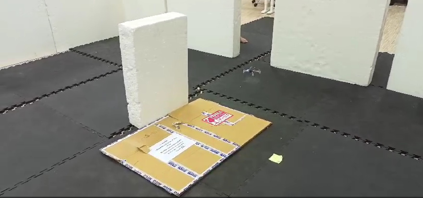
The optimized trajectory and command vectors were validated in both kinematic simulation and experimental quadrotor hardware setups.
Simulation Demonstration: 2D Drone Open-Loop Trajectory Planning and Obstacle Avoidance.
Hardware Demonstration: Real-time Trajectory Tracking and Avoidance Execution.
Simulation & Benchmark Results
Optimization metrics were benchmarked for the 5-second horizon under bounded acceleration constraints:
| Metric | Benchmark Result |
|---|---|
| Start State | $[p_x=0.0, p_y=0.0, v_x=0.0, v_y=0.0]$ |
| Goal State Target | $[p_x=10.0, p_y=8.0, v_x=0.0, v_y=0.0]$ |
| Planning Horizon | $N=20\text{ steps} \times \Delta t=0.25\text{ s} = 5.0\text{ seconds}$ |
| Obstacle Bounds | $[x_{\text{min}}, x_{\text{max}}] = [3.5, 6.2], [y_{\text{min}}, y_{\text{max}}] = [2.5, 5.5]$ |
| Acceleration Limits | $\vert{}a_x\vert{}, \vert{}a_y\vert{} \le 3.0\text{ m/s}^2$ |
| Terminal Position Error | $< 0.012\text{ meters}$ |
| Collision Clearance | Trajectory circumvents obstacle region without boundary violation |
Key Takeaways
- Formulated 2D quadrotor motion using linear double-integrator state-space models and exact RK4 matrix discretization.
- Transformed non-convex hard rectangular obstacle constraints into smooth, differentiable penalty fields using a 4-factor Softplus product formulation.
- Employed CasADi’s IPOPT interior-point solver to compute smooth, jerk-minimizing control inputs subject to strict saturation bounds ($\vert{}a\vert{} \le 3.0\text{ m/s}^2$).
- Verified trajectories across both simulation environments and real-world micro-UAV hardware setups.